Continuous Medial Representation
About
The continuous medial representation (cm-rep) is a framework for shape analysis and shape-based normalization. It is described in several papers, listed below. Essentially a cm-rep model is a 3D geometrical model that defines the skeleton and the boundary of an object at the same time. The term skeleton is synonymous to the medial axis, although medial axes usually are described for 2D objects and we are dealing with 3D objects. In 3D, the medial axis (skeleton) is a surface or a set of surfaces.
Cm-rep models are deformable. During deformation, the correct geometric relationship between the boundary and the skeleton is maintained. The skeleton of a deformed model is still the correct geometrical skeleton of the boundary of the deformed model. Also, during deformation, the topology of the skeleton (number of surfaces in the skeleton) does not change. In fact, in the code made public to date, only a single-surface skeleton is supported. Cm-rep models are used in a variety of biomedical applications.
Here is a list of papers that describe and use cm-reps.
- Neuroimage 2009: the most recent version of cm-rep, that uses the biharmonic equation to satisfy non-linear constraints.
- Neuroimage 2008: application of cm-rep to white matter tract modeling. Also describes model creation in more detail than other papers.
- Neuroimage 2007: describes the application of cm-reps to hippocampus-focused fMRI analysis
- IEEE TMI 2006: describes the first cm-rep approach to use partial differential equations to satisfy non-equality constraints. The theory is still relevant, but the actual approach has been superseded by the biharmonic approach (above).
Binary packages
We now make binary packages available for 64 bit Linux. Binaries are generated nightly from latest code in the CVS. Example data are included with the binary. Other platforms can be supported if there is demand; please do let us know. Use the link below to get the binaries.
Even if you use binaries, some installation is required. Specifically, see below about installing PARDISO, getting a PARDISO license, and setting up the environment.
Installation
Obtain cm-rep code from Sourceforge (https://sourceforge.net/scm/?type=cvs&group_id=250554).
Before compiling the cmrep code, you need install the following library first: ITK (http://www.itk.org/), VTK (http://www.vtk.org/), PARDISO (http://www.pardiso-project.org/) and the LAPACK library and G2C library.
cmrep code uses cmake (http://www.cmake.org/) to configure the compiler environment. Given the folder of the cmrep code is CMREP, it is suggested that you compile in a different folder, say CMREPBIN. To use cmake to configure, enter the folder CMREPBIN and then type
ccmake CMREP
For the configuration, cmake asks where the above required libraries are installed. You can ignore any warning messages. Once you specify all the required libraries and successfully generate the makefile from cmake. In the same folder, you can type
make
to compile and build cmrep executables. If you have compiling errors, you can go to the folder
CMREP/src/
and edit the line 2331 of file ScriptInterface.cxx
loc->FindClosestPoint(vox(0), vox(1), vox(2)); ==> loc->FindClosestPoint(vox.data_block());
You should be able to successfully compile now.
Description
The program cmrep_fit is used to fit a cm-rep template to a binary image (or in the future, to a grayscale image). You have to have a template to start with, and for the time being, I am still working on the code that generates templates, so you have to ask me (Paul) to create a template.
The fitting works in several stages. Usually, the first stages involve rigid or affine alignment of the model to the image, and the subsequent stages involve refining the model. The optimization parameters for each of the stages are specified in a parameter file. A typical parameter file is listed below.
Coordinate Systems and NIfTI
It is very important for users to be aware of the meaning of the coordinates through which cm-rep models are represented. The coordinates are in physical "RAS" space, with x increasing from left to right, y increasing from posterior to anterior, and z from inferior to superior. When fitting to image data, the cm-rep tool will use the voxel-to-RAS transform from NIFTI headers (i.e., the sform field). You can print out this transform using the companion tool convert3d
c3d image.nii -info-full
Usage
To run the program, you have to pass in the parameter file (see below), the initial template, the target binary image, and the output directory. A subdirectory tree will be created in the output directory.
cmrep_fit: fit cm-rep to image
usage:
  cmrepfit [options] param.txt template.cmrep target.img output_dir
options:
  -s N   : Only run fitting stage N (first stage is stage 0)
Parameter File
The parameter file specifies how optimization will proceed. Below is an example parameter file. It is suitable for fitting a hippocampus segmentation from in vivo MRI, for example.
# CMREP Parameter File (for automatic fitting)

# Define default parameters (optimization term weights)
DefaultParameters.Mapping = Identity
DefaultParameters.ImageMatch = VolumeOverlap
DefaultParameters.MedialRegularityTerm.Weight = 1.0
DefaultParameters.BoundaryCurvaturePenaltyTerm.Weight = 0.05
DefaultParameters.BoundaryGradRPenaltyTerm.Weight = 0.25
DefaultParameters.BoundaryJacobianEnergyTerm.Weight = 0.1
DefaultParameters.BoundaryJacobianEnergyTerm.PenaltyA = 30
DefaultParameters.BoundaryJacobianEnergyTerm.PenaltyB = 80
DefaultParameters.RadiusPenaltyTerm.Weight = 0.5
DefaultParameters.AtomBadnessTerm.Weight = 0.0
DefaultParameters.MedialCurvaturePenaltyTerm.Weight = 0
DefaultParameters.MedialAnglesPenaltyTerm.Weight = 0

# Define optimization stages
Stage.ArraySize = 5

# Alignment stage
Stage.Element[0].Name = align
Stage.Element[0].Mode = AlignMoments
Stage.Element[1].Blur = 1.2

# Affine stage
Stage.Element[1].Name = affine
Stage.Element[1].Mode = FitToBinary
Stage.Element[1].Blur = 0.4
Stage.Element[1].MaxIterations = 400
Stage.Element[1].Parameters.Mapping = Affine

# First deformable stage
Stage.Element[2].Name = def1
Stage.Element[2].Mode = FitToBinary
Stage.Element[2].Blur = 0.4
Stage.Element[2].MaxIterations = 2000

# Second deformable stage
Stage.Element[3].Name = def2
Stage.Element[3].Mode = FitToBinary
Stage.Element[3].Blur = 0.25
Stage.Element[3].MaxIterations = 2000
Stage.Element[3].Refinement.Subdivision.Atoms = 0
Stage.Element[3].Refinement.Subdivision.Controls = 1

# Third deformable stage
Stage.Element[4].Name = def3
Stage.Element[4].Mode = FitToBinary
Stage.Element[4].Blur = 0.25
Stage.Element[4].MaxIterations = 2000
Stage.Element[4].Refinement.Subdivision.Atoms = 1
Stage.Element[4].Refinement.Subdivision.Controls = 0
Stage.Element[4].Parameters.ImageMatch = BoundaryIntegral
The parameter file is a set of key/value pairs. The keys are organized into a hierarchical structure.
The parameter file essentially has two sections: default parameters and stage-by-stage definitions. At each stage, an optimization is performed. This optimization minimizes an objective function consisting of different terms, and the relative weights of these terms are specified as parameters to the optimization. Most of these parameters are the same for all stages so they are specified in the 'DefaultParameters' section. If you need to override one of the parameters in a given stage, you can do that by setting key/value pairs in 'Stage.Element[N].Parameters'. An example of that is in stage 4 above, where the key ImageMatch is overriden.
Stage Specification
As you see above, stages are specified as an array. First, the number of stages must be provided, as follows:
Stage.ArraySize = 5
Then, each stage is specified as a section 'Stage.Element[#]'. Within each stage section, the following keys can be defined.
- Name (required)
- The name of the stage. This should be a short name that is used to generate the output filenames associated with the stage. For example
- Mode (required)
- The optimization mode for the stage. Currently, there are only two modes, 'AlignMoments' and 'FitToBinary'. The first, 'AlignMoments' is for moments of inertia alignment, and is usually the very first stage in an optimization. It gets the model roughly aligned to the binary image. The other, 'FitToBinary' is used for all deformable optimization.
- Blur
- The amount of Gaussian smoothing to apply to the binary image in this optimization stage. The value is a floating point number that specifies the standard deviation of an isotropic Gaussian kernel, in millimeters. Usually, you want to blur more in the early stages of optimization, to keep the model from getting stuck in local minima. You always need some blurring, otherwise image gradient computation will not work.
- MaxIterations
- The maximum number of iterations at this stage. Default, if unspecified is 1000. For large models, 1000 iterations may not be enough for the optimization to converge.
- Refinement
- This section describes how the model is refined from the previous stage to the current. Usually during multi-stage optimization you want to do some refinement - i.e., start with a coarse model and make it finer by adding the number of control points. As the number of control points increases, you also want to increase the density at which the model is sampled. Since cmr_fit supports various types of medial models, the refinement has to be specified differently depending on the model type (cartesian vs. subdivision surface; brute force vs. pde-based)
- Refinement.Subdivision.Controls
- This is a refinement parameter for subdivision surface based models. It specifies the number of subdivisions applied to the control point mesh from the previous stage. For example, if at the previous stage the control point mesh had 40 vertices and 60 edges, and you set this value to 1, then at the beginning of the current stage, the control mesh will have 100 vertices and 120 edges (each edge is split by the subdivision). If you omit this parameter, no subdivision will take place.
- Refinement.Subdivision.Atoms
- This is a refinement parameter for subdivision surface based models. It specifies the number of subdivisions applied to the sampling mesh. The sampling mesh is the mesh that is used to compute image match and all other penalty terms in optimization. It is usually more dense than the control mesh.
- Parameters
- This section is used to override values specified in the DefaultParameters section.
Optimization Parameters
The following keys/values can be specified in DefaultParameters section or in the Parameters subsections of the stage sections.
- Mapping
- Defines the search space for optimization. Choices are Affine for global affine matching, Identity for searching over all parameters of the model, RadiusSubset for searching only over the radius scalar field, and PositionSubset for searching over the skeleton surface, but not the radius field. One more option is 'Reflection', which is used for fitting data that is symmetric across some plane. However, in most cases, Affine or Identity is used.
- ImageMatch
- Defines the way that the match between the model and binary image is computed. Options are VolumeOverlap and BoundaryIntegral. The first is best used in early and intermediate stages of optimization. It estimates the volumetric overlap between the model and the binary image. The second should be used once the model is very close to the target. It minimizes the image gradient along the boundary of the model.
- MedialRegularityTerm.Weight
- A floating point number giving the weight of the regularization prior on the medial surface. The prior penalizes distortion in the area element along the medial surface and is used to establish some degree of geometric correspondence between the initial template and the fitted template. Typically it can be set to 1.
- BoundaryCurvaturePenaltyTerm.Weight
- A penalty based on the curvature of the medial model's boundary. Should be used carefully, as there is a direct tradeoff between quality of fit and curvature. If the input binary image is fairly smooth already, set this to 0.
- BoundaryGradRPenaltyTerm.Weight
- This penalty should only be used for the 'BruteForce' medial models (as opposed to models based on solving a PDE). It uses a penalty to make sure that the Riemannian gradient of R (the radius field) has magnitude close to 1 along the edge of the medial surface. The value of 0.25 seems to work just fine.
- BoundaryJacobianEnergyTerm.Weight
- This penalty makes sure that the boundary of the model does not cross itself. You almost never have to play with the weight of this term (0.1 is fine). There are two other parameters related to this term, PenaltyA and PenaltyB. Ask me if you have problems with the jacobian penalty going to infinity and I can tell you how to adjust these parameters.
- RadiusPenaltyTerm.Weight
- Punishes radius field becoming negative. Never causes problems in my experience. Leave it set to 0.5.
- Other Weights
- Leave at zero. These are experimental and should not be used.
Template file
The template file is a text file with extension ".cmrep". Below is an example parameter file.
Grid.Type = LoopSubdivision
Grid.Model.SolverType = PDE
Grid.Model.Atom.SubdivisionLevel = 0
Grid.Model.Coefficient.FileName = def1.vtk
Grid.Model.Coefficient.FileType = VTK
Grid.Model.Coefficient.FileName specifies the cmrep model file.
Examples
The cmrep code contains a examples folder, which includes one parameter file(cmrparam_init.txt), one cmrep template file (def1.cmrep), one cmrep model file (def1.vtk) for hippocampus and two target segmentation files (fs_brain_hipp_L_manual.nii and fs_brain_hipp_R_manual.nii) to be fitted with. To run the cmrep fitting, you can use the following command
CMREPBIN/cmrep_fit cmrparam_init.txt def1.cmrep fs_brain_hipp_L_manual.nii fs_brain_hipp_L
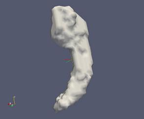
The output is saved in 3 subfolders (cmrep, image, and mesh) within the folder fs_brain_hipp_L. The final fitted cmrep surface is stored in the file def3.bnd.vtk in the mesh folder. For visualization, def3_target.vtk gives the surface of the target segmentation to be fitted. Using ParaView (http://www.paraview.org/), you can load these vtk files and check how the surfaces look like. Here is a tutorial on how to use ParaView. The following figure shows the initial cmrep medial model, def1.vtk,
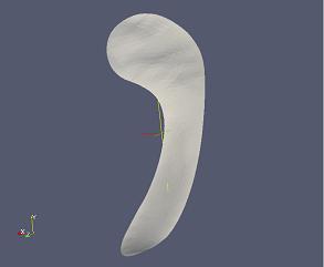 The initial medial model
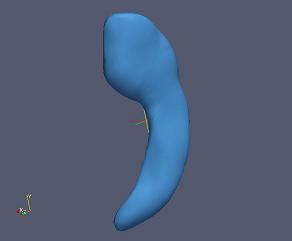
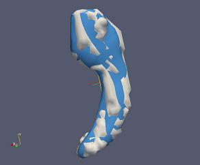
Here are the target hippocampus surface to be fitted and the fitted cm-rep surface. Both are generated by cmrep_fit. The overlap view is also given for a direct comparison.