Section 10. New in ITK-SNAP 2.0
This section describes the most important features added to ITK-SNAP since the main tutorial was written. This includes changes introduced in versions 1.2 through 2.0.
Multisession Support
When one ITK-SNAP session is running, you can open another ITK-SNAP session, without closing the first one. The two sessions will be synchronized. As you move the cursor in one ITK-SNAP session, the cursor will automatically move to the same anatomical location in all other open ITK-SNAP sessions.
How do you open multiple ITK-SNAP sessions? If you run ITK-SNAP from the command line, just execute the command you use to launch ITK-SNAP again when another session of ITK-SNAP is running. If you run ITK-SNAP using an icon or menu item, select that icon or menu item again.
 | On the MacOS operating system, you must run ITK-SNAP from the command line for multisession support to work. Open a terminal window and type /Applications/ITK-SNAP.app/Contents/MacOS/InsightSNAP |
Multisession support is particularly useful when working with multiple scans from the same MRI imaging session. Often, multiple scans are acquired with different imaging parameters and different slice orientations. For instance, one image may be sagittal, another image may be coronal, and a third image may be acquired in an oblique direction. If you open each image in a separate ITK-SNAP session, the cursor will always point to the same anatomical location in each session. The anatomical location is determined by the mapping from voxel coordinates to physical coordinates that is stored in the header of each image. Of course, these mappings must be correct for the multisession support to work.
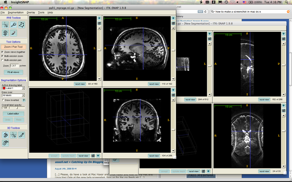
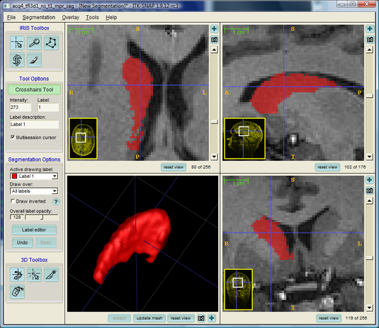
The image above shows two sessions of ITK-SNAP. One (in the front) is displaying an 7 Tesla MP-RAGE image, and the one in the back is displaying a T2-weighted image from the same session. The MP-RAGE image is sagittal, and the T2 image is oriented with slices approximately orthogonal to the long axis of the hippocampus. As you can see, the cursor points to the same anatomical coordinate in both images. However, each image is rendered in its native voxel space - there is no interpolation or resampling!
You can turn off cursor synchronization if you want the cursor in each ITK-SNAP version to operate independently. Select the crosshairs tool (press 1) and deselect Multisession Cursor. You can also disable synchronized zooming and panning, that is on by default. Select the zoom/pan tool (press 2) and deselect Multisession Zoom and Multisession Pan. These last two settings may be disabled permanently by going to Tools->Display Options->General and deselecting the corresponding checkboxes.
This feature was inspired by MRIcro.
Support for color images
Color images can be loaded into ITK-SNAP. A color image is simply a set of three images stored together in one file. The three images give the intensity of the red, green and blue components of the color image. We often refer to color images as RGB images.
| As of ITK-SNAP version 2.0, supported RGB image formats are NIfTI and MetaImage |
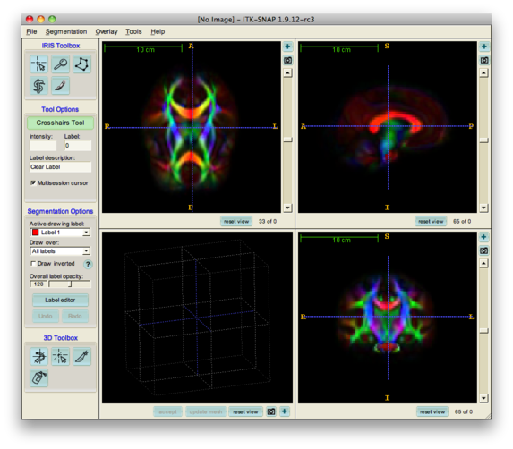
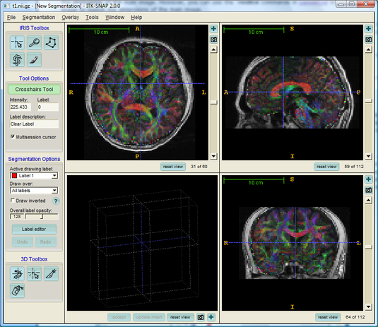
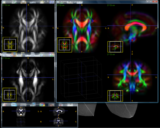
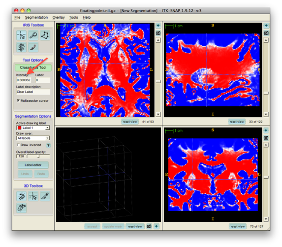
To open an RGB image, select File->Open RGB Image from the ITK-SNAP main menu. We have provided a sample RGB image in NIfTI format in the downloads area of this website. Here is what an RGB image looks like in ITK-SNAP:
You can inspect the values of the image's red, green and blue components in the layer inspector. You can invoke it by selecting Tools->Image Info.
You may notice that some of the functionality in ITK-SNAP is not available when viewing an RGB image. In particular, automatic segmentation with active contours is not available. But all of the manual segmentation tools are available. One of the applications of RGB image support in ITK-SNAP is to segment anatomical structures in diffusion tensor imaging (DTI) data. In fact, the image shown above is an example of a DTI dataset encoded as an RGB image, where the color describes the principal direction of diffusion (red: left to right; green: anterior to posterior; blue: superior to inferior), and the overall luminosity is scaled by the fractional anisotropy of the DTI data.
Support for floating point images
In older versions, ITK-SNAP expected the greyscale image to have integer values in the range -32768 to 32767. With version 1.8, we no longer require greyscale images to have values falling into a particular range. For example, a greyscale image may have floating point intensity values between -1 and 1. As you move the cursor in the image, ITK-SNAP will report a floating point intensity value.
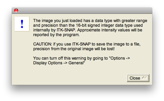
However, it is important to keep in mind that internally, ITK-SNAP represents greyscale images using 16-bit integers. If the image you load has values between -1 and 1, these values will be mapped to integers between -32768 and 32767. This mapping, of course, can affect the precision of your floating point data. In the example shown above, the true intensity value at the voxel under the cursor is 0.560364, whereas ITK-SNAP reports 0.560352. This is a limitation, but we felt it was an acceptable tradeoff for the memory and speed savings we get by representing images internally as short integers. If you need the precise intensity value at a voxel, use the -probe command in convert3d.
Because of the change in precision, ITK-SNAP displays a warning every time you open a floating-point image. In particular, it cautions that if you save the greyscale image to another file (or override the file you just opened), you will lose the precision from the original image.
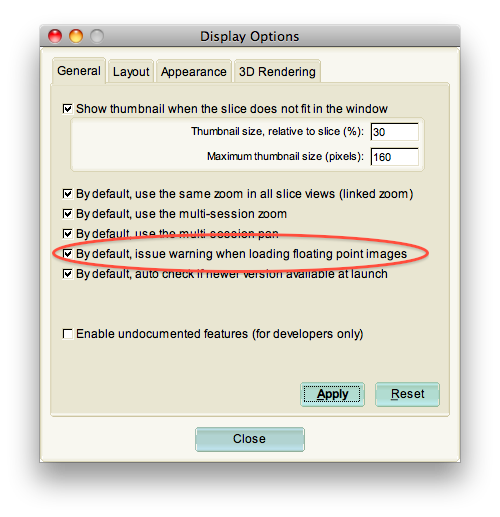
If you work frequently with floating point images, you may want to disable this message. This is done under Tools->Display Options.
Multiple image layers
In older versions, ITK-SNAP supported just two image layers: the greyscale image and a segmentation image. In version 2, you can have any number of image layers. Each image layer can be a grayscale image or an RGB image. The first image you load into ITK-SNAP is called the main image, and the subsequent images are called overlays. Overlays are always displayed on top of the main image layer. A typical application of overlays is to superimpose a statistical map on an anatomical image. The following are the key features of overlays:
- Overlays must have the same image dimensions as the main image. ITK-SNAP will not open overlays that do not match the dimensions of the main image. However, you can use the -reslice commands in convert3d to resample an overlay image to match the dimensions of the main image.
- Overlays should also have the same voxel space to physical space mapping (i.e., origin, voxel spacing, etc) as the main image. If they do not, ITK-SNAP will issue a warning, letting you know that the mapping in the overlay image will be ignored and replaced by the mapping from the main image.
- Multiple overlays can be loaded. The sequence is important. The main image is rendered first. The first overlay is rendered on top of the main image. Subsequent overlays are rendered on top of each other.
The segmentation image is treated internally as another image layer, the one that is rendered on top of all other image layers.
There is some redundancy between multisession support and support for multiple image layers. But there are very substantial differences between the two modes. Multisession support allows you to view multiple scans, each in its native voxel space, while maintaining linkage between selected voxels. Overlays are intended more to display data derived from the main image, such as statistical maps.
Layer Inspector: Intensity Contrast Adjustment
The layer inspector provides a new interface for changing the appearance of the main image and overlays. It included the intensity contrast adjustment functionality from early ITK-SNAP versions, but now makes it available for overlays as well. The layer inspector also allows you to change the color map used to render each layer, as well as to change its transparency. Lastly, the layer inspector provides information about each layer. Below is the layer inspector window opened to the image contrast adjustment tab.
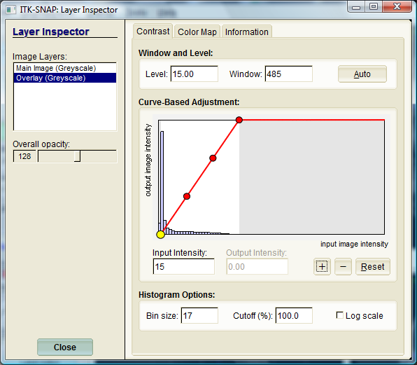
On the left of the window, the available image layers are listed. For each layer, overall opacity of the selected can be adjusted; setting opacity to zero will hide the selected layer. In the contrast adjustment page, you can specify the mapping from the intensity range of the input image (e.g., 0 to 4096) to the range of displayed intensities (0 to 1). For example, in the screenshot above, the intensity range 15 to 500 is mapped linearly to the range of displayed intensities. You can also specify a nonlinear mapping by moving the control points on intensity contrast mapping curve. The histogram of the selected layer is plotted to help make contrast adjustments. You can change the way the histogram is displayed, including bin size, vertical scaling, and log-vs-linear scale.
Intensity contrast adjustment is not available for RGB images.
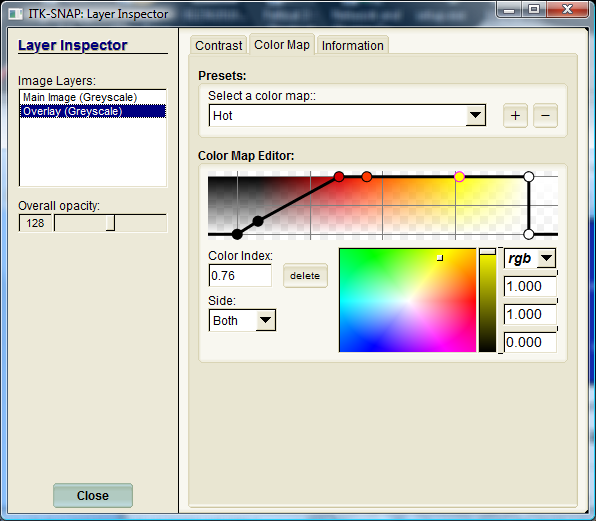
Layer Inspector: Color Map Adjustment
The screenshot above illustrates the new interface for color map selection and editing. The drop down list at the top allows you to select among a dozen or so color maps included in ITK-SNAP. You can also save your own color map in this list using the plus button.
The color map editor allows you to modify color maps. The color map is represented as a piecewise linear mapping from the range [0, 1] to the RGBA color space. We refer to the input value in the range [0 1] as the color index.
| Note that both the image contrast mapping and the color map are used together to determine the mapping from input image intensities to RGBA space! The intensity contrast curve maps input intensities to the color index. The color map then maps the color index to RGBA values. This approach allows you to reuse the same color map for many images. |
Let us examine the graphical display at the top of the color map editor closely. Think of this display as a graph, with the horizontal axis representing the input range [0, 1]. The vertical axis is the alpha (i.e., opacity) value. The bold black line gives the mapping from the input range to alpha. Values of color index below zero (first control point) have zero alpha (fully transparent); values between 0 and 0.35 (third control point) are semi-transparent; values from 0.35 to 1 are fully opaque; and values greater than 1 are fully transparent. Why do we explicitly define the opacity for color index values below 0 and above 1? This is important because some intensity values in the image may be mapped outside of the range [0, 1] by the intensity contrast curve. We want to be able to make these values transparent, e.g., when displaying statistical maps or other types of overlays.
You can change the alpha mapping by moving the control points up and down (changing their alpha value), as well as left and right (changing their color index). In addition, each control point has a color, which you can change using the color chooser provided. The color is interpolated between the control points, and shown in the background of the graphical display.
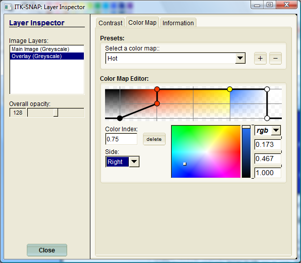
Each control point can be continuous or discontinuous. To make a control point discontinuous, change the Side drop down from Both to Left or Right. When you do so, you can edit just one side of the control point, creating a discontinuity in color, alpha or both. A color map with discontinuities is illustrated below. By default, color maps are discontinuous at 0 and 1 and continuous at all other control points.
You can add a new control point by clicking in the graphical color map display away from an existing control point. You can also delete a selected control point using the button provided.
| Notice that for the main image layer, the alpha values have no effect because the main layer is always fully opaque. Alpha values only apply to overlays. Color map adjustment is not available for RGB images. |
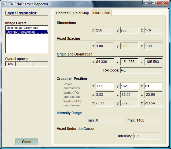
Layer Inspector: Information Pane
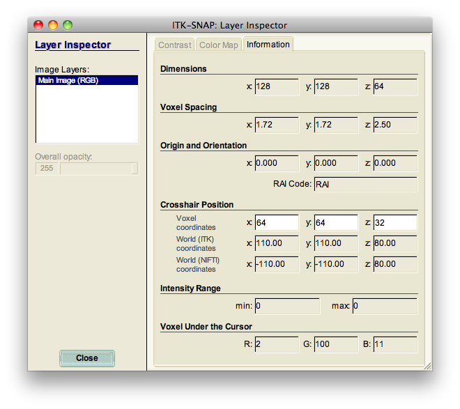
The last page in the layer inspector is the information pane. It gives general information about the image layer, as well as the value of the voxel under the cursor. Note that for RGB layers, the red, green and blue components of the image are listed.
Notice that extensive information is given about the cursor location. Three sets of coordinates are given: voxel coordinates, world coordinates (ITK coordinate frame), and world coordinates (NIfTI coordinate frame). ITK and DICOM use an RAI to LPS coordinate frame, where the x physical coordinate runs from right to left, the y coordinate runs from anterior to posterior and the z coordinate runs from inferior to superior. NIfTI and MNI use the LPI to RAS coordinate frame (x is left to right, y is posterior to anterior, z is inferior to superior).
Automatic contrast adjustment
A new feature is to perform contrast adjustment automatically. This is invoked using Alt-I on the keyboard (Command-I on the Mac) or using the Auto button in the image contrast adjustment interface. ITK-SNAP finds lower and upper quantiles of the image histogram to automatically set the contrast. This seems to work well for most images.
DICOM support
Users should note improved support for DICOM images, compared to earlier versions. When loading DICOM data, select File->Open Greyscale Image.. as you would for any other image file format.
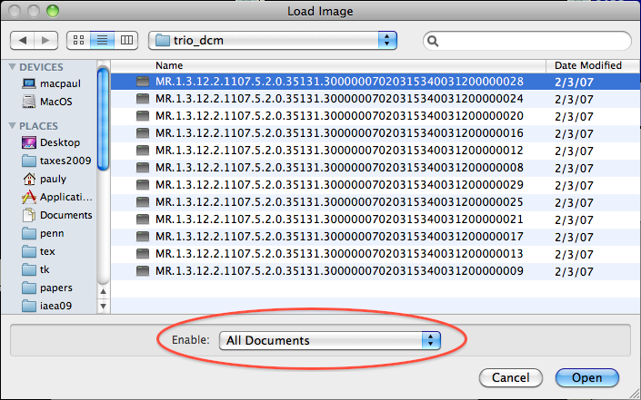
In the dialog that appears, select Browse, navigate to the DICOM directory, and select one of the files in that directory. Unless the file has a ".dcm" extension, the file browser may not show you any files in the directory containing the DICOM data. In that case, you need to tell the file browser dialog to show "All Documents" as opposed to the default of "All Image Files", as shown below.
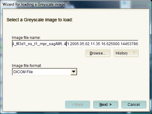
Usually, DICOM files have long filenames with lots of numbers. ITK-SNAP may not be able to automatically guess that the file is in DICOM format, so you may need to manually select DICOM under Image file format after you've browsed for a file.
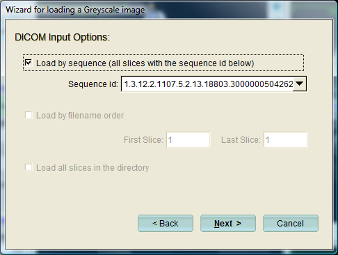
When you press Next, the following special dialog will appear:
This dialog displays all the sequences available in the DICOM directory. Each sequence typically corresponds to an image. Select one of the sequences, and press Next. After that, loading proceeds as usual.
For more advanced DICOM functionality, we recommend the DICOM to NIfTI converter dcm2nii, which is distributed as part of MRIcron.
Changing image orientation
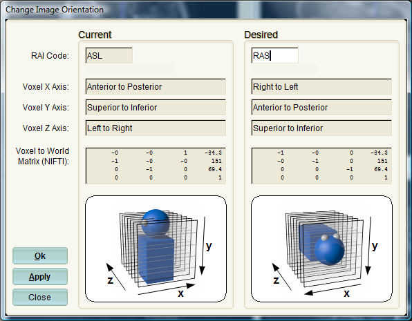
Sometimes the images you load into ITK-SNAP have wrong header information regarding image orientation (i.e., voxel space to physical space mapping). ITK-SNAP provides limited support for changing the orientation of the greyscale image. This is accomplished through the Tools->Reorient Image menu option.
The reorient image dialog shown above allows you to change image orientation by changing a three-letter orientation code. For example, above, we are changing the orientation from ASL to RAS. Below the codes, the explanation of the code is given. For example ASL means that the voxel x coordinate runs from anterior to posterior, and so on. The actual matrix mapping the voxel coordinates to NIfTI physical coordinates is given underneath. Lastly, a graphical representation of the three-letter code is given. For example, the ASL orientation has sagittal slices, and RAS has axial slices.
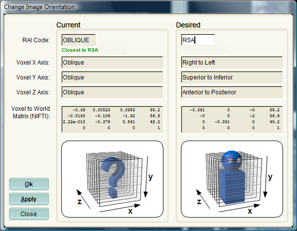
There are 48 possible 3-letter codes. Each code corresponds to the upper left 3x3 submatrix of the NIfTI matrix. To correspond to a letter code, the 3x3 matrix must have a simple form: a permutation of a diagonal matrix. Some images are acquired obliquely and have more complex NIfTI matrices. For these images, the 3-letter code closest to the orientation encoded in the NIfTI matrix is displayed (see below). However, when you reorient the image, you must select a 3-letter code; it is not possible to edit the NIfTI matrix directly.
Exporting segmentations as meshes
By default, segmentations are saved as multilabel images. However, you can also save a geometrical primitive mesh corresponding to a particular label. Select Segmentation->Save As Mesh. You will be prompted to select a label to export and the file format to save the mesh. We recommend using the VTK file format, which can be visualized and extensively edited using the Paraview suite.
Undo and redo
By popular demand, undo and redo functionality has been added. ITK-SNAP will keep a history of all changes made to the segmentation image layer, allowing you to restore the segmentation to an earlier state. Undo/redo is implemented by storing compressed difference images in memory, which allows quite a long (often unlimited) undo history without a large memory overhead. However, remember that Undo/Redo does not protect you from losing your work from crashes. Be sure to save your work often.
Extended keyboard shortcuts
We have added keyboard shortcuts for the most frequently used commands in ITK-SNAP. For most operations, you should be able to keep your mouse cursor inside the image display area, and not have to move it to press buttons in the UI.
Enhancements to image navigation and automatic panning
To minimize the need to switch between the Crosshairs mode and the Zoom/Pan mode, we added zoom and pan functionality to the Crosshairs mode. The mode now behaves as follows:
- Left mouse button moves the crosshairs (click or hold and drag).
- Right mouse button zooms (hold and drag up and down).
- Middle mouse button pans (hold and drag in all directions).
- Rotating the mouse wheel changes the slice.
Additionally, we implemented an automatic panning feature. When you zoom into an image and move the crosshairs by holding and dragging the left mouse button, the image will pan automatically as you move the cursor to the edge of the slice display window. This makes panning a lot easier than having to switch to the middle mouse button. The speed at which the image pans depends on how close you move the mouse cursor to the edge of the window.
Paintbrush mode with adaptive paintbrush
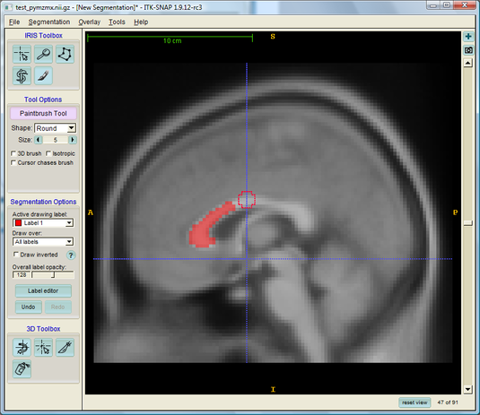
A paintbrush mode has been added to improve manual segmentation.
In paintbrush mode, you hold the left mouse button and drag the mouse to paint with the currently selected label over the image. The right mouse button acts as the eraser, painting with the clear label over the selected label. This allows you to quickly touch up a segmentation, or even to create segmentations from scratch.
By default the brush is two-dimensional, i.e., it paints only in the selected slice. You can choose to make it three-dimensional, so that adjacent slices are also affected. You can set the shape and size of the brush. When image voxels are anisotropic, you can choose to make the brush isotropic.
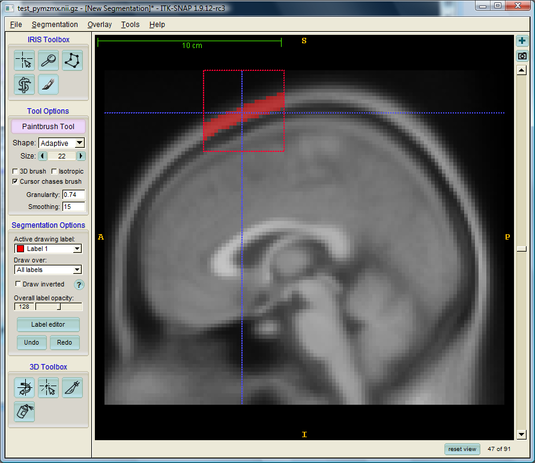
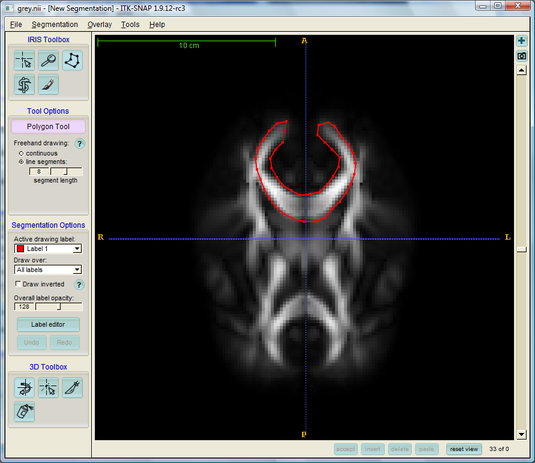
A powerful feature is the adaptive paintbrush, selectable under Shape. This paintbrush actually performs automatic segmentation inside the paintbrush. In the example below, it was used to label a part of the skull with just one click. The segmentation finds a contiguous block of voxels similar in appearance to the voxel under the cursor. The watershed segmentation algorithm in ITK is used internally. The adaptive paintbrush can be applied in 2D as well as 3D. Below, is an example of a quick and dirty segmentation of the caudate nucleus in routine MRI data. It was created using 6 mouse clicks with the 3D adaptive paintbrush.
Enhancements to the Polygon Drawing Mode
Polygon drawing is now more compatible with tablet devices. It supports freehand drawing, where you hold and drag the pointing device instead of making a series of clicks. In freehand drawing mode, you can choose to create a continuous curve, or to insert a series of polygon vertices at regularly spaced intervals. The latter can be subsequently edited.
Additionally, keyboard shortcuts were added for the accept, paste, insert, and delete buttons.
Layout organization
With new layout organization options, you can use screen space more efficiently and really take advantage of the multi-session features of ITK-SNAP 2.0.
These are the specific enhancements that are available:
- Expanded slice windows
- click the plus button in the upper right corner of each slice window (or 3D window) to expand the slice window. Click again to bring back all four windows.
- Hide UI components
- press F3 to toggle certain components of the user interface. You can make the slice views take up all of the screen area in the ITK-SNAP window.
- Fullscreen mode
- press F4 to enter and exit full screen mode.
Tools for preparing papers and presentations
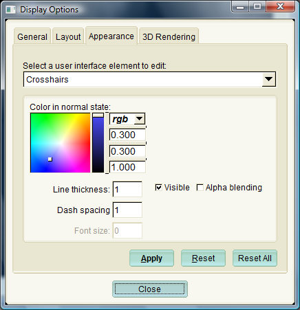
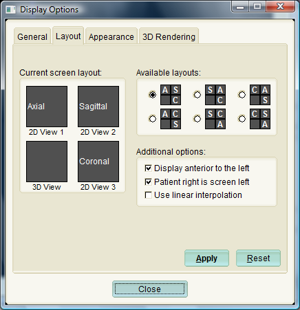
We often see screenshots taken in ITK-SNAP in papers and presentations. ITK-SNAP 2.0 offers a few new features to make paper and presentation preparation easier. You can customize the appearance of elements displayed in the slice windows and the 3D window. For example, you can hide the anatomical labels and the ruler, make the crosshairs thicker so that they are easier to see, and change the color of the background. This customization is available through the Appearance tab under Tools->Display Options. There is a Reset button that will restore settings to their defaults.
Some of the options under the other tabs of the Tools->Display Options dialog also affect appearance. For example, you can switch between nearest neighbor and linear interpolation of images under the Layout tab. You can also change the layout of the slice views and switch between neurological and radiological conventions.
Several options are available for saving screenshots in ITK-SNAP. In the upper right corner of each slice panel (and on the lower right of the 3D view panel), there is a small 'camera' button ( ) that takes a snapshot of that panel. The filename is generated automatically (snap0001.png), with the number incremented each time you save a screenshot. Screenshots generated by the camera button include all of the overlays and appearance elements in the slice panel; i.e., the cursor, anatomical labels, etc. What you see is what you get. The same functionality is also accessible through the File->Export->Screenshot menu.
In addition, you can create an animation by stepping through the slices in one of the slice panels and saving a screenshot for each slice. This is accessed through File->Export->Screenshot Series menu. You will be prompted for a directory where the screenshots will be saved.
Lastly, you can save just the slice of the main image layer without other layers and various graphical annotations. This is done using File->Export->Image Slice.
Interoperability with Convert3D
Convert3D is a great companion to ITK-SNAP. Convert3D is a command line tool that offers many image processing and analysis functions, which are not directly available in ITK-SNAP. For example, you can resample, resize and reslice images, perform image arithmetic, as well as do more complex operations such as bias field removal in MRI data. There are several scenarios where Convert3D can be complimentary to ITK-SNAP.
- Postprocessing segmentation images
- You can extract individual labels from an ITK-SNAP segmentation image and save them as binary images containing just a single label. You may do so using the -thresh command
c3d segmentation.nii.gz -thresh 5 5 1 0 -o label05.nii.gz
You may also do this for each label automatically.
c3d segmentation.nii.gz -split -o label%02d.nii.gz
- Preprocessing greyscale images
- Often, segmentation quality in MRI data can be improved by correcting for bias field inhomogeneity in the MRI. This functionality can be accessed through Convert3D with the -biascorr command. There are many other preprocessing operations that can be performed using Convert3D.
- Generating speed function images
- ITK-SNAP offers limited functionality for generating speed function images for active contour evolution (edge detection and region competition). Advanced users may generate their own speed images by applying filtering commands in Convert3D.
- Resampling overlay images to match main image
- Suppose you want to overlay an fMRI statistical map over an anatomical image. The two images are likely to be in the same space, but have different resolution. The difference in resolution prevents you from loading the statistical image as an overlay in ITK-SNAP. But you can resample the fMRI image using a simple Convert3D command
c3d anatomical.nii.gz fmristat.nii.gz -reslice-identity -o overlay.nii.gz
- Computing overlaps for reliability analysis
- Often you want to compare two segmentations of the same image by different raters. This is easily done using the -overlap command. Suppose the segmentations are named seg1.nii and seg2.nii and the labels you are interested in comparing are 10 and 15:
c3d seg1.nii seg2.nii -overlap 10 -overlap 15